Understanding Arc Length Parameterization with 🦏&🦗

0. Introduction

In the fields of multivariable calculus and differential geometry, the concept of “arc length parameterization” is extremely important. However, for many people, it may seem obscure and difficult to understand at first.

For example, in do Carmo’s Differential Geometry of Curves and Surfaces (Section 1.5), the definition of curvature is closely related to arc length:

Let $\alpha:I\to\mathbb{R}^3$ be a curve parameterized by arc length $s\in I$ . The number $\lvert \alpha''(s)\rvert=\kappa(s)$ is called the curvature of $\alpha$ at $s$ .

Similarly, in George Thomas’s Thomas Calculus (Section 13.3), arc length is used as a parameter to describe a curve:

$\mathbf{r}(s)=\cos(s/\sqrt{2})\mathbf{i}+\sin(s/\sqrt{2})\mathbf{j}+(s/\sqrt{2})\mathbf{k}$
… each value of determines a point on $C$ , and this way of describing $C$ using $s$ is what we call an arc length parameter for the curve.

Although this concept may seem complex at first, it is crucial for designing and understanding complex curves and shapes. I will attempt to explain this fascinating concept in a more vivid way using Rhino & Grasshopper.

📋1. Prerequisites

To better understand arc length parameterization, we need to review some basic mathematical knowledge:

1.1. Vector-Valued Functions

📝Definition 1: A vector-valued function is simply a function whose domain is a set of real numbers and whose range is a set of vectors. This means that for every number $t$ in the domain of $\mathbf{r}$ there is a unique vector in $V_3$ denoted by $\mathbf{r}(t)$ . If $f(t), g(t)$ and $h(t)$ are the components of the vector $\mathbf{r}(t)$ , then $f, g$ , and $h$ are real-valued functions called the component functions of $\mathbf{r}$ and we can write $\mathbf{r}(t)=\left< f(t),g(t),h(t)\right>=f(t)\mathbf{i}+g(t)\mathbf{j}+h(t)\mathbf{k}$

In simple terms, the distinctive feature of vector-valued functions is:

Input is a number
Output is a vector (three numbers)

🗃Example 1: The simplest vector-valued function is:

\mathbf{r}(t)= \begin{cases} f(t) &= t \\ g(t) &= t \\ h(t) &= t \\ \end{cases}

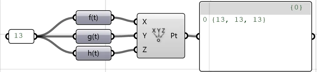
In Grasshopper, we can use the “🔋Construct Point” component to represent this. Therefore, when $t=13$ , we have $\displaystyle \mathbf{r}(13)=\begin{bmatrix}13\\13\\13\end{bmatrix}$ .

Note

In mathematics, vectors and points are different concepts. For simplicity, I will not strictly distinguish between them.

🗃Example 2: Let’s look at a slightly more complex example: a helix can be expressed using a vector-valued function.

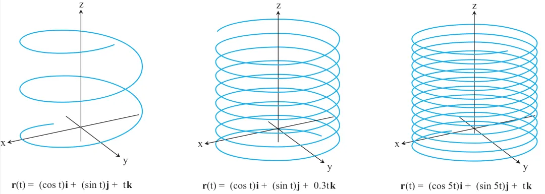(©️Thomas’ Calculus)

Similarly, it can be expressed in the system of linear equations:

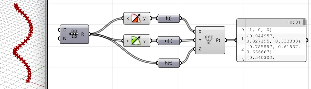
\begin{align} x &= \cos t \\ y &= \sin t \\ z &= t \\ \end{align}

We can use the “🔋Construct Point” component to represent this curve. Here, we can appreciate that when the output is a 3-vector, it is given a geometric meaning. I just need to give a single value $t$ to this function, and it will give me a point in space!😍When we give a sufficiently dense set of values, these points form a smooth curve.

1.2. Arc Length

The arc length not only represents the length of an “arc” but also the total length of a curve.

📝Definition 2: The arc length of a plane curve with parametric equations $\displaystyle x=f(t),y=g(t),a\leq t\leq b$ , as the limit of lengths of approximating polygonal paths and, for the case where $f'$ and $g'$ are continuous, we arrived at the formula $L=\int_a^b\sqrt{(\frac{dx}{dt})^2+(\frac{dy}{dt})^2}dt.$

If you have forgotten calculus and partial derivatives, don’t worry. The essence of this formula is that the total length of a curve can be obtained by dividing the curve into small segments and summing the lengths of each segment. When our division is infinitely fine, the result of this summation is the total length of the curve.

As shown in the figure, the blue curve is the curve we want to measure, and the red curve is the polygonal path used to approximate the blue curve.

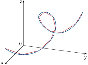
(©️Thomas’ Calculus)

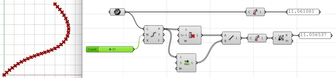
We can use a Grasshopper example to understand this. When our division is finer, the two curves’ lengths are closer.

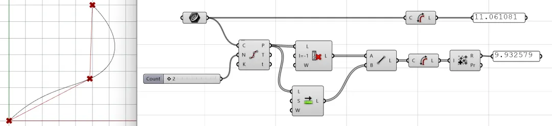
At this point, we can use trigonometric function to calculate the distance between two very close points:

\sqrt{(\frac{dx}{dt})^2+(\frac{dy}{dt})^2}.

2. What is Arc Length Parameterization?

After the above preparation, we finally need to discuss the essence of arc length parameterization🙌. From do Carmo’s Differential Geometry of Curves and Surfaces (Section 1.5), we know that:

Let $\alpha:I\to\mathbb{R}^3$ be a curve parameterized by arc length $s\in I$ . The number $\lvert \alpha''(s)\rvert=\kappa(s)$ is called the curvature of $\alpha$ at $s$ .

So, what is “arc length parameterization”, and what is “parameterized by arc length”?

Let’s review the helix example. The points on the helix are expressed as:

\mathbf{r}(t) = (\cos t)\mathbf{i} + (\sin t)\mathbf{k} + t\mathbf{k}.

Or:

\begin{align} x &= f(t) = \cos t \\ y &= g(t) = \sin t \\ z &= h(t) = t. \\ \end{align}

Notice that? All these expressions are with input $t$ . The $t$ is given, which belongs to the interval $I$ , i.e., $t\in I$ .

Remark

This $I$ is also the “🔋Domain” in Grasshopper.

Let’s try to use $\mathbf{r}$ to express the points on the curve. Suppose the input is $t$ , we then write: $\mathbf{r}(t)$ . In rigorous mathematical language, this is

A smooth curve $\mathbf{r}$ parametrized by $t$ .

Therefore, when we talk about “arc length parameterization” and “parameterized by arc length”, we are actually talking about ==replacing the input $t$ from to $s$ !==

That is, as long as we can find the relationship between $t$ and $s$ , we can re-interpret the curve using $s$ ! So, what can be used to establish the relationship between $s$ and $t$ ? The answer is arc length!💡

The arc length of $\mathbf{r}(t)$ is:

\begin{align} s(t) &= \int_a^t \sqrt{\left(\frac{df}{du}\right)^2 + \left(\frac{dg}{du}\right)^2 + \left(\frac{dh}{du}\right)^2} du \\ &= \int_0^t \sqrt{ (-\sin t)^2 + (\cos t)^2 + 1^2} du = \int_0^t \sqrt{2} du = \sqrt{2} t. \end{align}

Therefore, we can swap $s$ and $t$ :

\begin{align} s &= \sqrt{2} t \\ t &= s/\sqrt{2} \\ \end{align}

Then, substituting $t = s/\sqrt{2}$ into $\mathbf{r}(t)$ , we get the equation of the curve expressed using $s$ . This process is so-called “arc length parameterization”, and this curve is “parameterized by arc length”.

\begin{align} \mathbf{r}(t) &= \cos t\mathbf{i} + \sin t\mathbf{k} + t\mathbf{k} \\ \mathbf{r}(s(t)) &= \cos(s/\sqrt{2})\mathbf{i} + \sin(s/\sqrt{2})\mathbf{j} + (s/\sqrt{2})\mathbf{k} \end{align}

3. Verify in Grasshopper

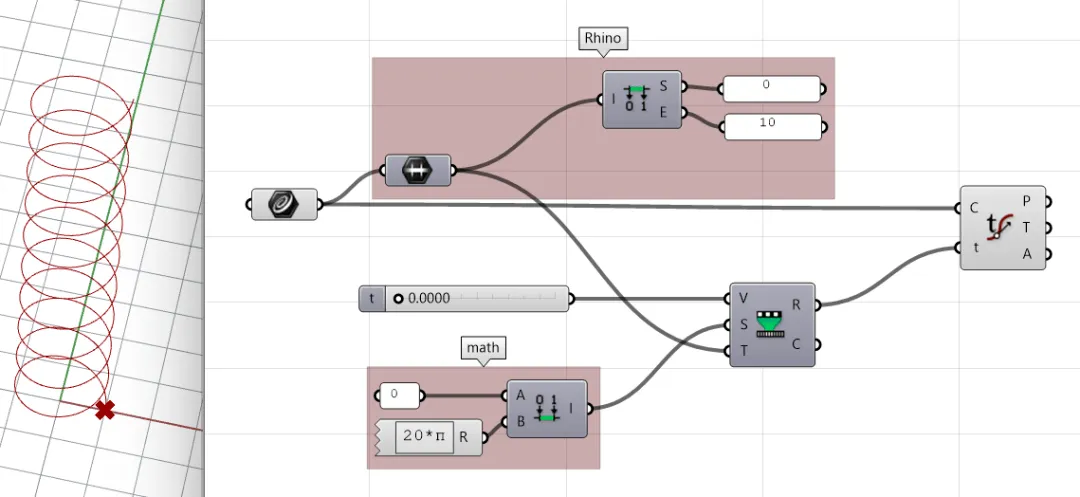
Now, let’s apply these theories to Grasshopper for practical operation. I drew a helix in Rhino, as shown below.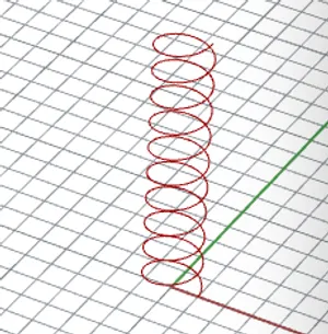

3.1. Curve Domain

First, we need to define the domain of the curve:

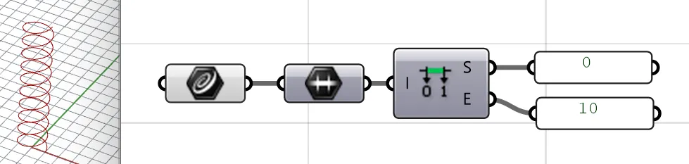
Here, we need to think about whether the interval $0\leq t \leq 10$ is we need. This interval is the definition domain of a Rhino.Geometry.Curve, but it may not be what we expect.

Let’s review the helix formula:

\mathbf{r}(t) = (\cos t)\mathbf{i} + (\sin t)\mathbf{j} + t\mathbf{k}.

Actually, its more general form is:

\mathbf{r}(t) = (a\cos t)\mathbf{i} + (a\sin t)\mathbf{j} + bt\mathbf{k}.

Here,

$a$ controls the rotation radius of the helix, and
$b$ controls the “how compressed” in the $z$ direction. At the same time, we see that $t$ is the parameter of the trigonometric function, therefore using radian as $t$ may be a good choice✔️. By observing how many turns this curve makes, we find that it has 10 turns! So, the interval of is:

0\leq t\leq 10 \times 2\pi.

We can use the “🔋Remap” component to map the $t$ from mathematical space to the domain of Rhino.Geometry.Curve.

$gh-remap-helix-from-math-to-rhino.png$

3.2. Curve Formula

Our objective🎯 is to figure out the values of $a$ and $b$ .

\mathbf{r}(t) = (a\cos t)\mathbf{i} + (a\sin t)\mathbf{j} + bt\mathbf{k}.

3.2.1. Calculate b

The value of $b$ is easy to calculate. The simplest method is to take $t=10\times2\pi$ . When $t=20\pi$ , the point has rotated 10 times and has reached the end of the interval. So, $z$ is:

z = 10 \times 2\pi b,

i.e., the end of the interval, also the end of the curve. We can simply get the value of $z$ :

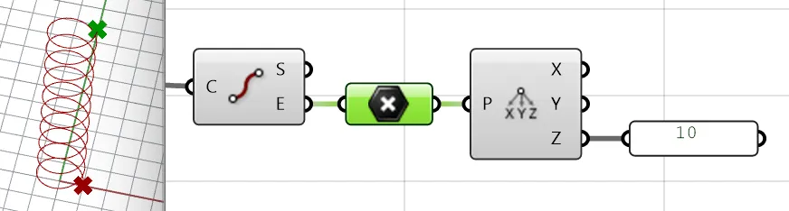
Thus, we can get:

\begin{align} 10 &= 10\times 2 \pi b \\ b &= \frac{1}{2\pi}. \end{align}

3.2.2. Calculate a

We can take any value $t$ , for example $t=3.3$ :

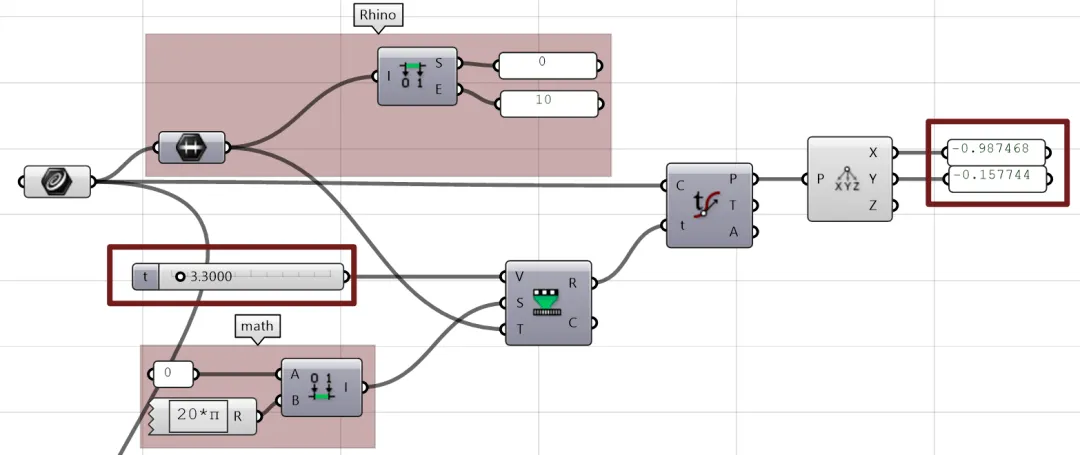
At this time, $x$ and $y$ are:

\begin{align} -0.987468 &= a \cos(3.3) \\ -0.157744 &= a \sin(3.3) \\ \end{align}

Squaring both sides, we get:

\begin{align} (-0.987468)^2 + (-0.157744)^2 &= a^2 \cos^2(3.3) + a^2 \sin^2(3.3)\\ (-0.987468)^2 + (-0.157744)^2 &= a^2 (\cos^2(3.3) + \sin^2(3.3))\\ a^2 &= 1 \end{align}

Because $a\geq1$ , we know that $a=1$ .

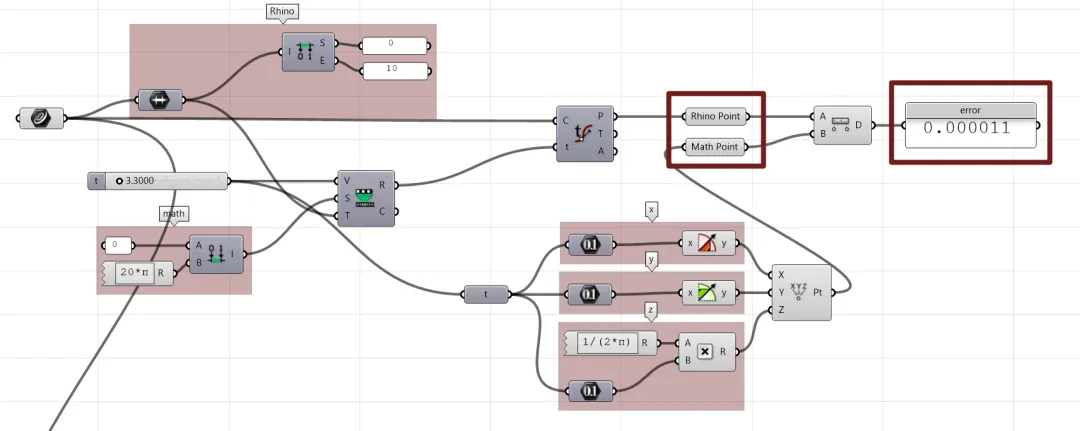
Rearranging, we get the formula for the helix. Now, let’s plug in the values of $a$ and $b$ :

\begin{align} \mathbf{r}(t) &= (1\cos t)\mathbf{i} + (1\sin t)\mathbf{j} + \frac{1}{2\pi}t\mathbf{k}\\ x&=\cos t \\ y&=\sin t \\ z&=\frac{1}{2\pi} t. \\ \end{align}

The results show that the distance between the points obtained through mathematical reasoning and those calculated by Rhino is within an acceptable tolerance.

$gh-error-math-very-small.png$

3.3. Reparameterization from t to Arc Length s

Next, let’s reparameterize the curve:

\mathbf{r}(t) = (1\cos t)\mathbf{i} + (1\sin t)\mathbf{j} + \frac{1}{2\pi}t\mathbf{k}.

First, we use the following formula to calculate the arc length and establish the relationship between $s$ and $t$ :

s(t) = \int_a^t \sqrt{\left(\frac{df}{du}\right)^2 + \left(\frac{dg}{du}\right)^2 + \left(\frac{dh}{du}\right)^2} du.

Substituting the formula, we get:

\begin{align} s(t) &= \int_a^t \sqrt{\left(\frac{df}{du}\right)^2 + \left(\frac{dg}{du}\right)^2 + \left(\frac{dh}{du}\right)^2} du \\ &= \int_a^t \sqrt{\left(-\sin t\right)^2 + \left(\cos t\right)^2 + \left(\frac{1}{2\pi}\right)^2} du = \int_0^t\sqrt{\frac{1}{4\pi^2}+1}du = \sqrt{\frac{1}{4\pi^2}+1}t \\ \end{align}

That is, the relationship between $s$ and $t$ is:

\begin{align} s &= \sqrt{\frac{1}{4\pi^2}+1}t \\ t &= \frac{1}{\sqrt{\frac{1}{4\pi^2}+1}}s \end{align}

So, if we express the helix curve using $s$ , it will be:

\begin{align} \mathbf{r}(s) &= \cos \left(\frac{1}{\sqrt{\frac{1}{4\pi^{2}} + 1}}s\right) \mathbf{i} + \sin\left( \frac{1}{\sqrt{\frac{1}{4\pi^{2}} + 1}}s \right)\mathbf{j} + \frac{1}{2\pi}\frac{1}{\sqrt{\frac{1}{4\pi^{2}} + 1}}s\mathbf{k}. \\ x &= \cos \left(\frac{1}{\sqrt{\frac{1}{4\pi^{2}} + 1}}s\right) \\ y &= \sin\left( \frac{1}{\sqrt{\frac{1}{4\pi^{2}} + 1}}s \right) \\ z &= \frac{1}{2\pi}\frac{1}{\sqrt{\frac{1}{4\pi^{2}} + 1}}s. \end{align}

We can also verify this using Grasshopper. The difference between the curve constructed using mathematical expressions and the curve calculated using “🔋Evaluate Length” is very small.

Remark

Here, the error is larger than before because it involves a lot of root calculations. For whom is interested can further research numerical analysis.

4.Conclusion

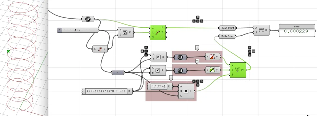
The example below is parameterized by $t$ :

\mathbf{r}(t) = \cos t\mathbf{i} + \sin t\mathbf{j} + t\mathbf{k}.

While the example below is parameterized by arc length $s$ :

\mathbf{r}(s) = \cos (s/\sqrt{2})\mathbf{i} + \sin (s/\sqrt{2})\mathbf{j} + (s/\sqrt{2})\mathbf{k}.

Through this detailed discussion and practice, we not only deepened our understanding of arc length parameterization but also implemented this concept in Grasshopper. This understanding and application provide us with powerful tools and perspectives for complex geometric modeling and problem-solving. I hope this article can help you apply these concepts in your own projects!