How to Derive the Policy Gradient with Monte Carlo Sampling?

A Review of the Objective

Let $\theta$ represent the parameters of our neural network, and let $\tau$ represent a specific trajectory sampled from the probability distribution of all possible trajectories, denoted by $p_\theta(\tau)$. Our goal is to find the optimal parameter $\theta^\star$ that maximize our expected value.

We define our objective function, $J(\theta)$, as the expected reward over these trajectories:

To maximize this expected value, we need to find the gradient of $J(\theta)$ with respect to $\theta$. We will show that this gradient can be expressed in a form that allows for estimation via Monte Carlo sampling.

Calculating the Gradient of $J(\theta)$

Because expected values represent a statistical average over a continuous space of trajectories, we can express $J(\theta)$ formally using an integral:

We compute the gradient of $J(\theta)$ with respect to $\theta$ by taking the derivative of the integral. Assuming we can pass the gradient operator inside the integral, we see that:

To evaluate this integral numerically, one might initially consider Riemann sum. In a standard Riemann sum for an integral $\displaystyle \int f(x)dx$, we evaluate the function at specific points and multiply by a small width $\Delta x$.

Applied to our trajectory space, we would slice the space of $\tau$ into small chunks $\Delta\tau$, yielding:

However, the space of possible trajectories is infinitely vast (encompassing all possible joint positions, velocities, and timestamps). Therefore, evaluating a Riemann sum over this space is computationally infeasible.

Monte Carlo Sampling

Because we cannot evaluate the integral analytically or via a Riemann sum, we turn to Monte Carlo sampling. To use Monte Carlo estimation, our integral must be structured as an expected value:

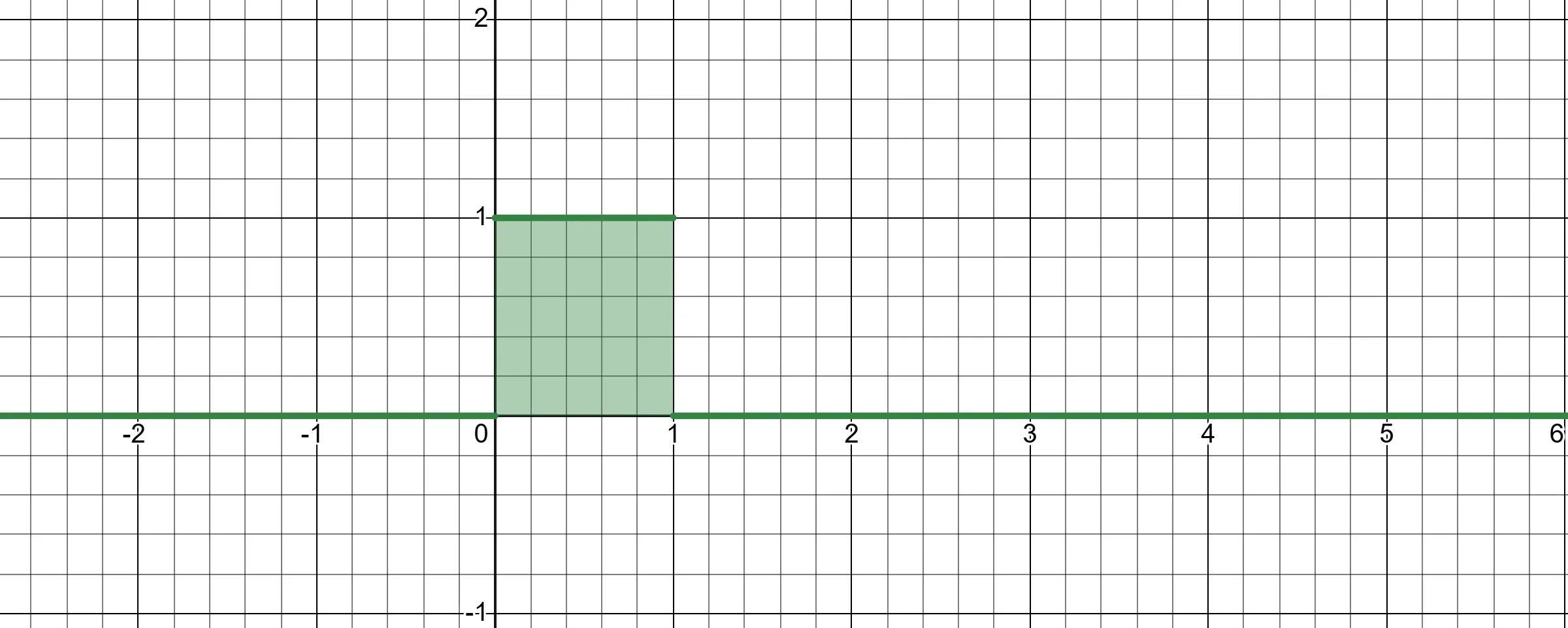
To illustrate, suppose we want to find the expected value of the function $f(x) = x^2$, where $x$ is uniformly distributed between 0 and 1. Here, our valid probability distribution is the probability density function $p(x) = 1$ for $x \in [0, 1]$, illustrated below.

Formally, we write this expected value as:

Because $p(x) = 1$, the exact analytical solution is:

If the function were too complex to integrate analytically, Monte Carlo sampling allows us to approximate the expected value by simulating it. We sample $N$ random values from our distribution and average the results:

Here is a brief Python script demonstrating this approximation:

import random
from collections.abc import Callable
 
def square(x: float) -> float:
    return x**2
 
def uniform_sample(lower: float, upper: float) -> float:
    return random.uniform(lower, upper)
 
def monte_carlo_sampling(
    sampler: Callable[[float, float], float],
    value: Callable[[float], float],
    sample_count: int,
) -> float:
    total = 0.0
    for _ in range(sample_count):
        x = sampler(0.0, 1.0)
        total += value(x)
    return total / sample_count
 
print(monte_carlo_sampling(uniform_sample, square, 1_000_000))

Running this code yields a result very close to $0.333$, demonstrating the power of the Monte Carlo method.

The Log Derivative Trick

Returning to our policy gradient, we encounter a problem. Our current gradient expression is:

This does not fit the Monte Carlo template because $\textcolor{red}{\nabla_\theta p_\theta(\tau)}$ is a gradient, not a valid probability distribution. To resolve this, we utilize a calculus identity known as the log-derivative trick.

Recall that by the chain rule, the derivative of the natural logarithm of a function $f(x)$ is:

If we substitute $\theta$ for $x$ and $p_\theta(\tau)$ for $f(x)$, we obtain:

Multiplying both sides by $p_\theta(\tau)$ yields our identity:

We can now substitute this identity back into our gradient integral:

Because the integral is now the product of a valid probability distribution ($p_\theta(\tau)$) and a specific value ($\nabla_\theta \log p_\theta(\tau) r(\tau)$), we can rewrite it as an expected value:

Expanding the Probability of a Trajectory

Next, we must expand the $\log p_\theta(\tau)$ term. The probability of a specific trajectory $\tau$ occurring is the product of the initial state probability and the probabilities of all subsequent actions and state transitions:

Consider the the product rule of logarithm gives:

we know that taking the natural logarithm of both sides transforms the products into sums:

We then apply the gradient with respect to $\theta$ to this entire expression:

Crucially, the terms $p(\mathbf{s}_1)$ and $p(\mathbf{s}_{t+1} | \mathbf{s}_t, \mathbf{a}_t)$ represent the dynamics of the environment. Because they do not depend on our network parameters $\theta$, their gradients with respect to $\theta$ are zero. This allows us to cancel them out:

leaving

The Final Gradient of $J(\theta)$

Finally, we substitute our expanded $\nabla_\theta \log p_\theta(\tau)$ expression and the expanded reward $r(\tau)$ back into our expected value equation.

This gives us the final, computable form of the policy gradient: