Why the Gymnasium API Looks the Way It Does?

Probabilistic Graphical Model

Let’s review what a graphical model looks like.

First, take a look at the node.

• $s$ denotes the state.
• $o$ denotes the observation.
• $p$ denotes the probability distribution.
• $\pi$ denotes the policy where $\theta$ the policy’s parameters.

Next, take a look at the edge:

• the edge between state $s_1$ to observation $o_1$ represents a stochastic process (a “sensor model”), which may or may not capture all the information from state $s_1$
• the edge from observation $o_1$ to action $a_1$ represents the policy.
• the edge between state $s_1$ and future state $s_2$ a transitional probability, also known as “dynamics”.

The gymnasium Code Snippet

Let’s look at this basic example from gymnasium.

import gymnasium as gym
env = gym.make("CartPole-v1", render_mode="human")
observation, info = env.reset()
episode_over = False
total_reward = 0
while not episode_over:
    action = env.action_space.sample()
    observation, reward, terminated, truncated, info = env.step(action)
    total_reward += reward
    episode_over = terminated or truncated
env.close()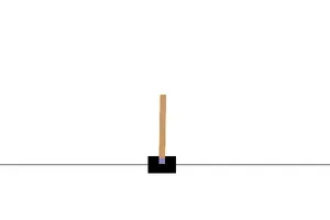

Even without an explanation, you can infer some reinforcement learning patterns just by looking at the variable names and control flows.

• action
• observation
• reward
• step

Now, let’s combine this with the math and dive deeper.

To the next state

Let’s focus on this specific line of Python

observation, reward, terminated, truncated, info = env.step(action)

💬Question We can ask a few key questions here:

• what represents the “sampling” ($\sim$) from the distribution $p$?
• what represents $s_{t+1}$?

🗣Answer The env.step() method acts as the sampler. It decides the next state based on the environment’s transition probabilities.

Identifying $s_{t+1}$ is a bit tricky. In short, the observation returned by this function corresponds to $o_{t+1}$. However, depending on the environment, this observation might effectively be the state:

• if $s_{t+1} = o_{t+1}$, it is a MDP (fully observed).
• if $s_{t+1} \neq o_{t+1}$, it is a POMDP (partially observed).

In an environment like CartPole, the system is fully observed. We can actually verify this by comparing the observation to the internal state:

observation, reward, terminated, truncated, info = env.step(action)
print(f"observation: {observation}")
print(f"state: {env.unwrapped.state}")
 
# The output shows they are identical:
# observation: [ 0.02138549  0.61995554  0.06039844 -0.7173455 ]
# state: [ 0.02138549  0.61995552  0.06039844 -0.71734546]

The Markov Property in Code

In the graphical model, we know that the states satisfy an important property called Markov property. This simply states that “the future state depends only on the present state”: $\mathbf{s}_{t+1} \perp \mathbf{s}_{t-1} | \mathbf{s}_t$

The expression above is read as “the state $\mathbf{s}_{t+1}$ and the state $\mathbf{s}_{t-1}$ are [conditional independence|conditionally independent] given($|$) the state $\mathbf{s}_{t}$”. ^965f65

Since the Markov property holds, we can clearly see which function signature is correct:

• ✅env.step(action)
• ❌env.step(action, previous_history_list)

The “God View” vs. The “Pixel View”

Let’s use Pong as an example to illustrate the difference between POMDP and MDP.

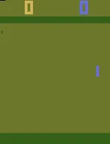
According to the documentation, the observation space of Pong is an image:

observation_space=Box(0, 255, (210, 160, 3), np.uint8)

Therefore, the agent cannot “understand” the full world state like it does in CartPole. In math terms, this means $o_t$ (the pixels) is not $s_t$ (the state). For example, looking at a single static image of Pong, you cannot tell if the ball is moving left or right. This is why we need to use technique like “frame stacking” to reconstruct the velocity components of the hidden state $s_t$ from partial information.

We can compare them like this:

	CartPole	Pong
illustration
observation space	Cart Position, Cart Velocity, Pole Angle, Pole Angular Velocity	RGB Image
type	fully observed (MDP)	partially observed (POMDP)