A Visual Guide to Hand-Eye Camera Calibration in Robotics

Notation

Let’s establish our notation first.

Remark

This note follows the notation convention from the Introduction to Robotics: Mechanics and Control and Russ Tedrake.

The term

${}^A X^B$

means “the pose of frame $\Set{B}$ measured in frame $\Set{A}$”.

Example

Suppose the position of $\Set{B}$ measured from $\Set{A}$ is $1, 0.5, 0.5$, then ${}^A X^B$ can be written as ${}^A X^B =\begin{bmatrix}0.0 & -1.0 & 0.0 & 1.0 \\ 1.0 & 0.0 & 0.0 & 0.5 \\ 0.0 & 0.0 & 1.0 & 0.5 \\ 0.0 & 0.0 & 0.0 & 1.0 \end{bmatrix}$

Composition follows the frame labels mathematically:

Tip

Hint: we normally read the transformation from right to left.

• $C \to A$
• $C \to B, B\to A$

Remark

You can think of $X$ as a homogeneous transformation matrix or a rigid motion.

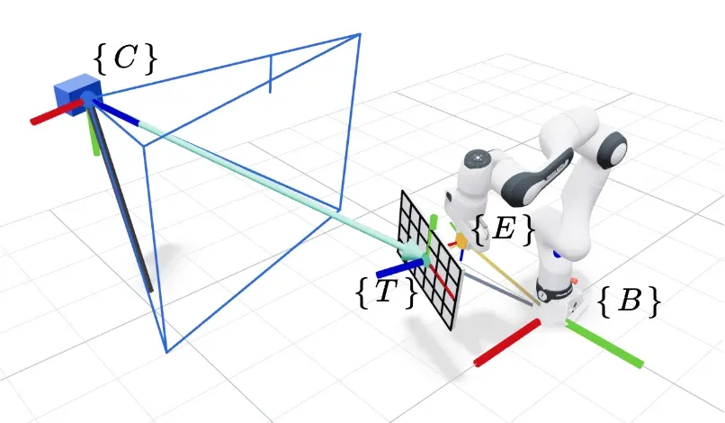
Frames

For camera calibration using a robot, we define the following frames.

• $B$: Robot Base frame
• $E$: Robot Effector frame
• $C$: Camera optical frame
• $T$: ArUco/ChArUco target frame

Remark

I’ll use eye-to-hand as the primary example, but the core math also works for eye-in-hand. I’ll leave applying this logic to eye-in-hand as an exercise for you. 😆

Known Transformation

During calibration, we record multiple samples. Let’s use $i$ to denote an arbitrary sample.

The transformation

is known. It represents the pose of end-effector measured from the robot’s base. We can easily obtain this via robot’s forward kinematics.

The transformation $^C X^{T_i}$ is also known. It represents the ChArUco/ArUco target frame measured from the camera’s optical frame.

How does the $^C X^{T_i}$ output the same unit (e.g., meter) as $^B X^{E_i}$?

Before calibrating, we have to fill out some configuration values. Notice the parameters “longest board size” and “measured marker size”. These refer to the physical dimensions you measure in reality. The camera detects the marker in pixel space, but using the camera’s intrinsics and these known physical dimensions, the algorithm sclaes the detection into physical units that match the robot’s coordinate system.

Does precision matter?

Absolutely! You can measure the board with a ruler. But for high-precision calibration, exact tolerances are crucial. This is why professional calibration boards (like this one) can sell up to $143!

Unknown Transformation

The transformation

is unknown. It refers to the camera frame measured from the robot base frame.Finding this is the entire goal of eye-to-hand calibration.

The transformation

is unknown and it refers to the ArUco/ChAruCo target frame measured from the end-effector frame.

Tip

The good news is this transformation is fixed as long as the gripper firmly grasps this board.

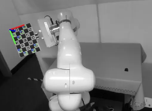
Example

Here’s an example how ChAruco can be detected and referred as target frame $\Set{T}$.

How Do We Solve it?

Thinking mathematically, we have 2 unknowns and 2 knowns. To solve this, our intuition tell us we need to construct a system of equations.

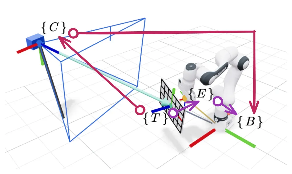
Looking at the physical setup, we define the target pose ${}^B X^T$ through two different paths:

• Path 1 (Through the arm): $B \to E \to T$ which is $^B X^{E} \cdot {}^E X^T$
• Path 2 (Through the camera): $B \to C \to T$ which is $^B X^C \cdot {}^C X^{T}$

Recall the composition rule we mention above that two homogeneous transformation matrices can be written as

Since both paths end at the exact same physical target in space, we can equate them:

where both sides are $^B X^T$.

Look closely at this equivalent transformation:

$^B X^{E_i} \cdot {}^E X^T = {}^B X^C \cdot {}^C X^{T_i}.$

It contains 2 unknowns ($^E X^T$ and $^B X^C$). However, $^B X^C$ (the camera pose) is the only one we actually care about. The ChArUco/ArUco board offset $^E X^T$ in the gripper is just a fixed “nuisance parameter” blocking our way.

Therefore, our mathematical strategy is to cancel out $^E X^T$ completely so we are only left with the camera pose.

To do this, we need a second equation. If we take two distinct samples, we can use one to isolate the nuisance parameter and substitute it into the other, effectively erasing $^E X^T$ from our math entirely.

Let’s see how this variable elimination works. Suppose we take two different poses, $i$ and $j$, giving us two equations:

We can isolate $^E X^T$ in the first equation by multiplying both sides by the inverse of the end-effector pose:

Next, we substitute this isolated $^E X^T$ into the second equation for sample $j$:

Now, we rearrange the terms to isolate the relative motions. Multiply the right side by $(^C X^{T_i})^{-1}$:

Let’s take a careful look on the last equation:

Notice that both bracketed terms describe a relative motion between the 2 samples:

• Let $A = {}^B X^{E_j} \cdot (^{B} X^{E_i})^{-1}$ . This is the relative motion measured by the robot.
• Let $B = {}^C X^{T_j} \cdot (^{C} X^{T_i})^{-1}$ . This is the relative motion measured by the camera.
• Let $X = {}^B X^C$ . This is the static unknown camera pose we want to find.

We have successfully derived the most famous equation in hand-eye calibration:

$A X = X B.$

Remark

I’ll unveil the conceptual solution here, but to deeply understand this, I recommend two materials:

• Hand to sensor calibration: A geometrical interpretation of the matrix equation AX=XB
• screw theory

Let’s clarify the terminology:

• A Sample (or Pose): This is a single, static snapshot. The robot stops moving, and the camera takes a single picture of the marker. Normally you would click the “Take Sample” button.
• A Relative Motion: This is the physical movement between 2 samples. For example, the ${}^B X^{E_j} \cdot (^{B} X^{E_i})^{-1}$ is a relative motion between 2 samples.
• An Equation: In the $AX = XB$ format, one equation represents exactly one relative motion.

To solve $X$, we at least need

• 3 distinct samples
• 2 relative motions

Remark

When taking these samples, the motions must occur around different physical axes. Curious why? The screw theory explains everything!

Now let’s use $i, j, k$ to denote 3 samples. We then have 2 relative motions:

where the known relative motions are defined as:

• Motion 1: $A_1 = {}^B X^{E_j} \cdot (^{B} X^{E_i})^{-1}$ and $B_1 = {}^C X^{T_j} \cdot (^{C} X^{T_i})^{-1}$
• Motion 2: $A_2 = {}^B X^{E_k} \cdot (^{B} X^{E_j})^{-1}$ and $B_2 = {}^C X^{T_k} \cdot (^{C} X^{T_j})^{-1}$

If the math only strictly requires 3 samples, why do MoveIt and ROS tutorials usually ask you to collect 15 to 20?

In a mathematically perfect simulation, $A_1 X = X B_1$ and $A_2 X = X B_2$ are fully sufficient to lock down the 6 degrees of freedom. However, in physical reality, our knowns are flawed. The robot joints have tiny physical deflections (making $A$ noisy), and the camera has limited resolution and lighting artifacts (making $B$ noisy).

To combat this noise, we generalize this into an over-determined system of $N$ equations:

By collecting many samples across diverse angles and rotations throughout the robot’s workspace, we feed all these $A_m X = X B_m$ equations into an optimization algorithm (such as the Tsai-Lenz method).

In short, instead of looking for a “perfect” $X$, we minimize the error to pursue an optimal $X$.