Value Function: From Gridworld to Bellman Equation

Why is it important?

In Richard Sutton and Andrew Barto’s Reinforcement Learning: An Introduction, they write:

Quote

The concepts of value and value functions are the key features of the reinforcement learning methods that we consider in this book.

At first, I read this as: value functions are the whole center of RL. That was too narrow. Value functions are central to many classic RL methods, especially dynamic programming, Monte Carlo method, and temporal difference learning. But they are not the only way to think about RL.

After reading Lilian Weng’s blog post A (Long) Peek into Reinforcement Learning, I started to see a broader picture. RL methods can also be grouped by whether they learn a value function, a policy, or a model of the environment.

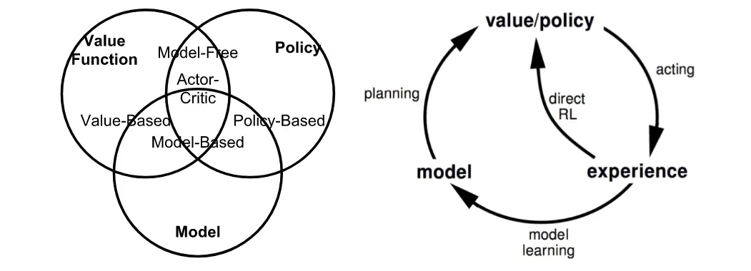
So my updated understanding is: Value functions are a central idea in many classic RL methods, but they are not the only object an RL algorithm can learn. A better way to classify RL algorithms is to ask 2 questions:

Does the agent use the model of the environment?
What does the agent learn: a value function, a policy, a model, or some combination of them?

I’ll leave these questions for the future me to answer. In the meantime, I also recommend the diagram of the taxonomy of RL Algorithms in OpenAI Spinning Up:

Intuition on Value Function

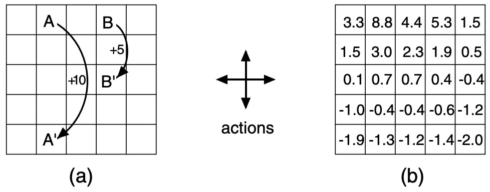
I want to use the “Example 3.8 GridWorld” in Reinforcement Learning: An Introduction to build intuition for the value function.

The rules of GridWorld game are as follows.

(1) Actions

From any cell, the agent can choose 1 of 4 actions:

north
south
west
east

Each action tries to move the agent one cell in that direction.

(2) Border

If the next state would be outside the grid, the agent stays in the same cell and receives reward -1.

(3) Special States

If the agent is in cell A , any action you moves it to A' and gives reward +10.
If the agent is in cell B , any action you moves it to B' and gives reward +5.

(4) Normal States

All other valid moves give reward 0.

The value of a state means the expected discounted future reward starting from that state, under a given policy. In this example, the policy is the random policy: each action has probability $1\over4$ .

Looking at figure (b), we can form the following intuition:

Cells A and B have the highest values because they give special positive rewards.
Cells near A and B also have relatively high values because the agent may reach those special states soon.
Cells near the wall have lower values because the agent has a higher chance hitting the border and receiving -1.

From Value Function to Bellman Equation

Let’s walk through the derivation of value function and the Bellman equation mentioned in the Reinforcement Learning: An Introduction.

\begin{align} V^\pi(s) &= \mathbb{E}_\pi\{R_t \mid s_t = s\} \\ &= \mathbb{E}_\pi\left\{\sum_{k=0}^{\infty} \gamma^k r_{t+k+1} \;\middle|\; s_t = s\right\} \\ &= \mathbb{E}_\pi\left\{r_{t+1} + \gamma \sum_{k=0}^{\infty} \gamma^k r_{t+k+2} \;\middle|\; s_t = s\right\} \\ &= \sum_a \pi(s,a) \sum_{s'} \mathcal{P}^a_{ss'} \left[\mathcal{R}^a_{ss'} + \gamma\, \mathbb{E}_\pi\left\{\sum_{k=0}^{\infty} \gamma^k r_{t+k+2} \;\middle|\; s_{t+1} = s'\right\}\right] \\ &= \sum_a \pi(s,a) \sum_{s'} \mathcal{P}^a_{ss'} \left[\mathcal{R}^a_{ss'} + \gamma V^\pi(s')\right] \end{align}

Here’s my updated notation based on my reading mixing up Reinforcement Learning: An Introduction, Algorithms for Decision Making, OpenAI Spinning Up, and David Silver’s course in UCL.

\begin{align} V^\pi(s) &= \mathbb{E}_\pi\{G_t \mid S_t = s\} \\ &= \mathbb{E}_\pi\left[\sum_{k=0}^{\infty} \gamma^k R_{t+k+1} \;\middle|\; S_t = s\right] \\ &= \mathbb{E}_\pi\left[R_{t+1} + \gamma \sum_{k=0}^{\infty} \gamma^k R_{t+k+2} \;\middle|\; S_t = s\right] \\ &= \sum_a \pi(a|s) \sum_{s'} \mathcal{P}^a_{ss'} \left[\mathcal{R}^a_{ss'} + \gamma\, \mathbb{E}_\pi\left[\sum_{k=0}^{\infty} \gamma^k R_{t+k+2} \;\middle|\; S_{t+1} = s'\right]\right] \\ &= \sum_a \pi(a|s) \sum_{s'} \mathcal{P}^a_{ss'} \left[\mathcal{R}^a_{ss'} + \gamma V^\pi(s')\right] \end{align}

Remark

The notation is slightly different from the original Sutton’s notation.

I will use $G_t$ for the return and $R_{t+1}$ for the one-step reward. This avoids mixing up “reward” and “return”.

The return is $G_t=R_{t+1}+\gamma R_{t+2} + \gamma^2 R_{t+3}+ \cdots = \sum_{k=0}^{\infty}\gamma^k R_{t+k+1}.$

The discount factor is $\gamma \in [0,1]$ .

We also have this equivalent notations:

$P^a_{ss'} = P(S_{t+1}=s' \mid S_t=s, A_t=a)$

$\mathcal{R}^a_{ss'} = \mathbb{E}[R_{t+1} \mid S_t=s, A_t=a, S_{t+1}=s']$

Let’s break down each step.

(1) $V^\pi(s) = \mathbb{E}_\pi[G_t \mid S_t = s]$

The value of state $s$ following the policy $\pi$ is denoted as $V^{\pi}(s)$ . It is equal to the expected return $\mathbb{E}_{\pi}$ of the “total discounted reward” (or simply “return” $G_t$ ) starting from state $s$ .

In simple words: the value function tells us how good it is to be in a state, measured by future reward.

(2) Why do we need $\gamma$ ?

Look at the equation $G_t=R_{t+1}+\gamma R_{t+2} + \gamma^2 R_{t+3}+ \cdots = \sum_{k=0}^{\infty}\gamma^k R_{t+k+1},$ we might raise this question.

The reason is that the reward sequence may never stop for continuing tasks. If the agent receives reward $R>0$ forever and $\gamma = 1$ , then

G_t = R + R + R + \cdots = \infty.

But with $0\leq\gamma\leq1$ , we have

G_t = R + \gamma R + \gamma^2 R + \cdots = \frac{r}{1-\gamma},

and therefore the return becomes finite.

Remark

However, we need to note that $\gamma=1$ can still be valid for tasks that always terminate.

To conclude, the point is not “we always need $\gamma < 1$ ”, but rather discounting helps make infinite-horizon returns well-defined and also makes many Bellman updates converge nicely.

(3) Recursive structure

The key step is the $\displaystyle G_t = R_{t+1} + \gamma G_{t+1}$ from

V^{\pi}(s) = \mathbb{E}_\pi [R_{t+1} + \gamma G_{t+1} \mid S_t =s].

This is where the recursive structure appears. The return from now is the immediate reward plus the discounted return from the next state. This is the heart of the Bellman equation.

Remark

The $\displaystyle G_t = R_{t+1} + \gamma G_{t+1}$ also refers to Bellman backup which essentially is: the reward-plus-next-value.

(4) Expanding over actions and next states

The expression

\begin{align} &\sum_a \pi(a \mid s) \sum_{s'} \mathcal{P}^a_{ss'} \left[\mathcal{R}^a_{ss'} + \gamma \, \underbrace{\mathbb{E}_\pi\left[\sum_{k=0}^{\infty} \gamma^k R_{t+k+2} \;\middle|\; S_{t+1} = s'\right]}_{V^{\pi}(s')}\right] \\ = &\sum_a \pi(a \mid s) \sum_{s'} \mathcal{P}^a_{ss'} \left[\mathcal{R}^a_{ss'} + \gamma V^\pi(s')\right] \end{align}

means:

first, average over all possible actions $a$ , according to the policy $\pi(a \mid s)$ .
then, average over all possible next states $s'$ , according to the transition probability $\mathcal{P}^a_{ss'}$ .
for each transition, add the immediate reward and the discounted value of the next state.

Remark

One minor but critical detail on the Sutton’s notation $\pi(s, a).$
Its modern equivalent is $\pi(a \mid s).$ Meaning, the probability distribution over action $a$ conditioned on state $s$ .

(5) Bellman Equation

Finally, we have the Bellman equation. I intentionally list out the variations I have seen as followed.

Reinforcement Learning: An Introduction:

V^{\pi}(s) = \sum_a \pi(s,a) \sum_{s'} \mathcal{P}^a_{ss'} \left[\mathcal{R}^a_{ss'} + \gamma V^\pi(s')\right]

OpenAI Spinning Up:

V^{\pi}(s) = \mathop{\mathbb{E}}\limits_{\substack{a \sim \pi \\ s' \sim P}} \left[ r(s, a) + \gamma V^{\pi}(s') \right]

David Silver:

V(s) = \mathbb{E} [R_{t+1} + \gamma V(S_{t+1}) \vert S_t = s]

Policy Evaluation

Let’s get our hands dirty.

The following code is my practice for evaluating the GridWorld environment. I asked kimi to write the skeleton of the quiz, leaving the step and policy_eval_sweep functions empty.

You can run this using uv run this-file.py

# /// script
# requires-python = ">=3.10"
# dependencies = [
#  "numpy",
# ]
# ///
import numpy as np
 
# Environment Setup
ROWS, COLS = 5, 5
GAMMA = 0.9
ACTIONS = [(-1, 0), (1, 0), (0, -1), (0, 1)]  # up,down,left,right
 
# Special States
A = (0, 1)
Ap = (4, 1)
B = (0, 3)
Bp = (2, 3)
 
def step(current_row, current_col, action) -> tuple[int, int, float]:
    if (current_row, current_col) == A:
        return (*Ap, 10.0)
    if (current_row, current_col) == B:
        return (*Bp, 5.0)
 
    delta_row, delta_col = action
    next_row = current_row + delta_row
    next_col = current_col + delta_col
    out_of_board = (
        next_row < 0 or next_row >= ROWS or
        next_col < 0 or next_col >= COLS
    )
    if (out_of_board):
        return (current_row, current_col, -1.0)
 
    return (next_row, next_col, 0.0)
 
def policy_eval_sweep(V_old: np.ndarray) -> np.ndarray:
    V_new = np.zeros_like(V_old)
    for row in range(ROWS):
        for col in range(COLS):
            total = 0.0
            for action in ACTIONS:
                update_row, update_col, immediate_reward = step(row, col, action)
                total += immediate_reward + GAMMA * V_old[update_row, update_col]
            V_new[row, col] = total / len(ACTIONS)
    return V_new
 
 
# Initialize
V = np.zeros((ROWS, COLS))
theta = 1e-5
 
# Log
history = {0: V.copy()}
history_steps = [1, 2, 3, 10]
 
for k in range(1, 10_000):
    V_new = policy_eval_sweep(V)
    delta = np.max(np.abs(V_new - V))
    V = V_new
    if k in history_steps:
        history[k] = V.copy()
    if delta < theta:
        print(f"converged after {k} sweeps")
        history_steps.append(k)
        history[k] = V.copy()
        break
 
# Print grid
def print_grid(V: np.ndarray, title: str, decimals: int = 1) -> None:
    print(f"\n=== {title} ===")
    # Check with fig 3.5(b) in RL-Sutton
    for r in range(ROWS):
        row_str = ""
        for c in range(COLS):
            val = V[r, c]
            if abs(val) < 0.05:
                row_str += f" {0:5.1f} "
            else:
                row_str += f" {val:5.1f} "
        print(row_str)
 
# show key steps
converged_step = history_steps[-1]
for k in history_steps:
    if k == converged_step:
        print_grid(history[k], f"k = {k} (converged)")
    else:
        print_grid(history[k], f"k = {k}")
 
# compare with Figure 3.5(b)
print("\n=== compare with Figure 3.5(b) (converged) ===")
figure_3_5_b = np.array([
    [3.3, 8.8, 4.4, 5.3, 1.5],
    [1.5, 3.0, 2.3, 1.9, 0.5],
    [0.1, 0.7, 0.7, 0.4, -0.4],
    [-1.0, -0.4, -0.4, -0.6, -1.2],
    [-1.9, -1.3, -1.2, -1.4, -2.0]
])
print("Result")
print(np.round(history[converged_step], 1))
print("\n Figure 3.5(b):")
print(figure_3_5_b)
print("\n error(should be 0):")
print(np.round(history[converged_step], 1) - figure_3_5_b)

Running this will yield an output that tracks the value propagation, converging at step 68.

=== k = 1 ===
  -0.5   10.0   -0.2    5.0   -0.5 
  -0.2    0.0    0.0    0.0   -0.2 
  -0.2    0.0    0.0    0.0   -0.2 
  -0.2    0.0    0.0    0.0   -0.2 
  -0.5   -0.2   -0.2   -0.2   -0.5 

=== k = 2 ===
   1.5    9.8    3.1    5.0    0.3 
  -0.5    2.2   -0.1    1.1   -0.5 
  -0.4   -0.1    0.0   -0.1   -0.4 
  -0.5   -0.1   -0.1   -0.1   -0.5 
  -0.8   -0.5   -0.4   -0.5   -0.8 

=== k = 3 ===
   2.3    9.6    3.8    4.9    0.7 
   0.4    2.1    1.4    1.0   -0.1 
  -0.6    0.4   -0.1    0.1   -0.6 
  -0.7   -0.2   -0.1   -0.2   -0.7 
  -1.1   -0.7   -0.6   -0.7   -1.1 

=== k = 10 ===
   3.3    8.9    4.4    5.3    1.4 
   1.5    3.0    2.2    1.8    0.5 
   0.0    0.7    0.7    0.3   -0.4 
  -0.9   -0.4   -0.3   -0.5   -1.1 
  -1.8   -1.3   -1.1   -1.3   -1.8 

=== k = 68 (converged) ===
   3.3    8.8    4.4    5.3    1.5 
   1.5    3.0    2.3    1.9    0.5 
   0.1    0.7    0.7    0.4   -0.4 
  -1.0   -0.4   -0.4   -0.6   -1.2 
  -1.9   -1.3   -1.2   -1.4   -2.0

Lookahead

After I worked with kimi, I tried to find whether any textbook covers this algorithm directly. It turns out yes. I found a close version in Chapter 7 of Algorithms for Decision Making by Mykel J. Kochenderfer.

In Sutton’s book, the Bellman equation is defined as

V^{\pi}(s) = \sum_a \pi(s,a) \sum_{s'} \mathcal{P}^a_{ss'} \left[\mathcal{R}^a_{ss'} + \gamma V^\pi(s')\right].

Kochenderfer directly provides a computational method for finding this value function iteratively, known as iterative policy evaluation. Each step uses a look ahead equation:

U_{k+1}^{\pi} (s) = R(s,\pi(s)) + \gamma \sum_{s'} T(s' | s,\pi(s)) U_{k}^{\pi}(s').

Remark

The $U$ here stands for “utility.” You can conceptually replace $U$ with Sutton’s $V$ , and $T$ (transition probability) with $\mathcal{P}$ .

Because this update rule is a contraction mapping, it is mathematically guaranteed to converge, resulting in the final equation:

U^{\pi} (s) = R(s,\pi(s)) + \gamma \sum_{s'} T(s' | s,\pi(s)) U^{\pi}(s').

Now let’s enjoy the beauty of implementing this in julia:

function lookahead(𝒫::MDP, U::Vector, s, a)
    𝒮, T, R, γ = 𝒫.𝒮, 𝒫.T, 𝒫.R, 𝒫.γ
    return R(s,a) + γ*sum(T(s,a,s′)*U[i] for (i,s′) in enumerate(𝒮))
end
 
function iterative_policy_evaluation(𝒫::MDP, π, k_max)
    𝒮, T, R, γ = 𝒫.𝒮, 𝒫.T, 𝒫.R, 𝒫.γ
    U = [0.0 for s in 𝒮]
    for k in 1:k_max
        U = [lookahead(𝒫, U, s, π(s)) for s in 𝒮]
    end
    return U
end

A few notes on this code:

U = [0.0 for s in 𝒮] initializes all state values to 0 at the beginning.
U = [lookahead(𝒫, U, s, π(s)) for s in 𝒮] takes the previous values as input and computes the new updated values.
γ*sum(T(s,a,s′)*U[i] for (i,s′) in enumerate(𝒮)) is the most interesting part. Even though we iterate through all possible states $\mathcal{S}$ , the transition probability function $T(s' | s, a)$ is not necessarily nonzero. Therefore, impossible states are naturally zeroed out and neglected.

Another way to write the lookahead function is to treat U as a function rather than a vector:

function lookahead(𝒫::MDP, U, s, a)
    𝒮, T, R, γ = 𝒫.𝒮, 𝒫.T, 𝒫.R, 𝒫.γ
    return R(s,a) + γ*sum(T(s,a,s′)*U(s′) for s′ in 𝒮)
end

Treating U as a function aligns much closer to the pure mathematical definition, while using U as a vector is easier to conceptualize and compute in discrete, finite-state environments like GridWorld.

In short,

$U$ -as-function is the math-friendly conceptual interface.
$U$ -as-vector is the efficient tabular implementation.

Value Function: From Gridworld to Bellman Equation

Why is it important?

Intuition on Value Function

(1) Actions

(2) Border

(3) Special States

(4) Normal States

From Value Function to Bellman Equation

(1) Vπ(s)=Eπ[Gt∣St=s]V^\pi(s) = \mathbb{E}_\pi[G_t \mid S_t = s]Vπ(s)=Eπ​[Gt​∣St​=s]

(2) Why do we need γ\gammaγ?

(3) Recursive structure

(4) Expanding over actions and next states

(5) Bellman Equation

Policy Evaluation

Lookahead

See also...

(1) $V^\pi(s) = \mathbb{E}_\pi[G_t \mid S_t = s]$

(2) Why do we need $\gamma$ ?