 Xingxin on Bug
 In this post, I’ll try to explain 📄Real-Time Execution of Action Chunking Flow Policies by Kevin Black et al. The authors later proposed a training-time version in 📄Training-Time Action Conditioning for Efficient Real-Time Chunking, but this post focuses only on the original inference-time method.
Prerequisites
We first review several ideas that appear throughout the paper.
Action Chunking
I first learned about action chunking from Tony Z. Zhao et al.’s paper, 📄Learning Fine-Grained Bimanual Manipulation with Low-Cost Hardware.
In a classic MDP, an agent outputs one action from the current state . In a POMDP, it usually acts from observation instead.
An action-chunking policy
outputs a sequence of future actions
rather than only one action .
TipThis is the dominant approach by 2026-07-08. Since the inference costs quite a lot of time. Therefore, outputs a chunk of action saves the GPU inference time.
We call the as the prediction chunk and as the execution chunk, meaning the number of actions sent to the controller. Usually, the execution chunk is often shorter, i.e., .
RemarkAn empirical ratio is which is used in 📄Diffusion Policy: Visuomotor Policy Learning via Action Diffusion, pi0, and pi05.
WarningThe original paper uses for the execution horizon. But I prefer to avoid confusion to the state .
Flow Matching
Many continuous-action robot policies use Flow Matching to generate action chunks.
To generate a chunk, we first sample Gaussian noise
A useful mental picture is:

A trained neural network predicts a velocity field.
Its inputs are
- the current noisy or partially denoised chunk ,
- the observation , and
- the flow time , Its output is a velocity field which has the same shape as the action chunk (make it flow🍃).
With Euler steps, one update is
The is the flow-matching time, and is the number of integration steps.
Intuitively, the learned velocity field moves the initial random noise toward a meaningful action chunk.

RemarkFor a more detailed introduction, see A Beginner’s Guide to Flow Matching.
TipRobot policies often use a small number of flow steps , such as 4, 5, or 8. The exact value depends on the model.
What does real-time mean?
As you might notice, there is a word “real-time” in the title. How to define it then🤔?
Let
- be the sampling period of the learned policy or controller, and
- be the time required to generate an action chunk.
Then a system is real-time only if it can generate an action chunk () with respect to the input (received ) within the fixed time constraint (), i.e., .
ExampleSuppose the learned policy runs at 50 Hz, so If my measured OpenPI inference time is about then the model cannot finish within one policy period. It is not real-time🚫 since
60ms > 20ms.By contrast, the control rate of Franka Research 3 robot is 1KHz and therefore the . The ruckig: Motion Generation for Robots and Machines can manage to generate action chunks around 250.
Therefore, we know that real-time is is possible✅ in
ruckigsince250µs < 1ms.
RemarkThe frequency of the learned policy could be considered as the dataset action sampling rate during teleoperation. In practice, the robot might run in low-level controller with 1KHz but the sampled dataset could be 50Hz or even smaller 20Hz.
Because these are different layers of the control stack, comparisons should be interpreted carefully‼️.
Synchronous Inference
This is the simplest way to deploy an action-chunking policy on a robot. The robot executes the current chunk, reaches the end of its execution horizon, starts the next inference call, and waits for the new chunk to finish.
When , this creates visible pauses between chunks. The pauses have 2 main effects:
- The robot takes longer to complete the task.
- The robot dynamics during evaluation differ from the dynamics in the training data.
RemarkSynchronous inference is the a common baseline for policies such as π0, π0.5, 📄OpenVLA: An Open-Source Vision-Language-Action Model, 📄Octo: An Open-Source Generalist Robot Policy, 📄RT-2: Vision-Language-Action Models Transfer Web Knowledge to Robotic Control, etc.
The second effect is especially problematic. Consider the following comparison:
| Training | Evaluation |
|---|---|
Suppose a demonstration contains a smooth motion.
- During training, the joint velocity changes naturally along the trajectory.
- During synchronous evaluation, however, the robot may be forced to hold its position while waiting for the next chunk, i.e., .
Therefore,
and a distribution shift is introduced👎️. The policy may never have seen this stop-and-restart behavior in its training data.
Asynchronous Inference
Synchronous inference wastes time by making the robot wait. A natural next step is asynchronous inference: generate the next chunk in the background while the current chunk is still being executed.
✒Notation 1: Define the inference delay as the number of controller timesteps between when is received and when is available:
where denotes floor function.
✒Notation 2: Let denote the action for world time inside the chunk generated from observation . It’s position inside that chunk is .
When Should the Next Inference Start?
Suppose is currently executing and we want to switch chunks after controller steps. Since inference takes steps, the next inference call must start at
Then the new chunk is ready at the desired switch time which ensures real-time constraint.
For a repeating asynchronous schedule, the useful feasibility condition is
- ensures that inference does not need to start before the current cycle begin.
- ensures the previous chunk contains enough future actions to cover the delay while the next chunk is being generated.
Tip😮💨Sounds confusing? No worries! The example will clear them out!
WarningHowever, asynchronous execution alone does not guarantee a smooth transition. While generating , the policy does not know exactly what will happen during the next controller steps. Therefore, the transition may be discontinuous and out of distribution.
See more in the coming section.
Alright, enough formulas, let’s use a concrete example. Suppose:
and choose:
We can digest everything with this diagram.

1️⃣ The First Chunk
The first chunk is
It is conditioned on the observation at time . For example, is the action intended for world time , predicted from .
2️⃣ When should asynchronous inference start?
Since the inference takes controller steps and we want to switch at , therefore we need to start the next inference call at
After the controller has executed and received , it starts generating
The new chunk becomes available at world time .
3️⃣ Which actions are not used?
There are 2 groups of unused actions which are marked in yellow.
From , the actions
are not executed because we switch after actions.
From , the actions
arrive too late. By the time is available, world time has already reached .
4️⃣ Which actions does the controller execute?
From the global world-time viewpoint, the controller executes
Notice that is the fifth entry of when using zero-based indexing.
5️⃣ Why can this sequence be problematic?
The transition
might be discontinuous. The two chunks were generated from different observations and may represent different valid strategies.
The author provides a nice diagram to illustrate this:
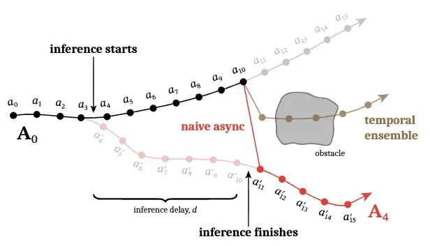
© Black et al.
Sometimes, it is coincident that the policy generates action chunks diverged at the inference timestep😮💨. In the diagram, the old chunk plans to move above the obstacle, while the new chunk plans to move below it.
Both chunks may be valid on their own, but switching between them in the middle of the motion can create a large jump in velocity or acceleration. This mismatch leads to jerky and unpredictable behavior⚠️.
The Big Picture of Real-time Chunking
Real-time chunking aims to keep the benefits of asynchronous inference while removing discontinuities at chunk boundaries.
No formulas yet. Just take a look at the big picture:

The transition is a useful startup example. After that, inference calls start every steps. The call after therefore starts at and generates .
📌Gap
Naive asynchronous inference may cause a discontinuous transition at the chunk boundary, e.g. to as indicated with red arrow.
📌Objectives
The objectives for the inference-time real-time action chunking algorithm are twofold:
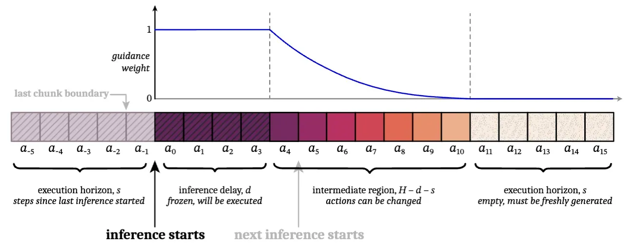
- Give the first overlapping entries full guidance as indicated with blue arrows.
- Leave the non-overlapping tail generated freely.
That’s it! That is the big picture and we will explain piece by piece in the remaining sections.
Real-Time Chunking as an Inpainting Problem
The novelty of this paper is to conceive of chunk generation as inpainting. Here’s the mindmap:

For the steady-state RTC example, let’s define the current chunk as
and the next chunk as
Intuitively, the first -steps in the chunk can be thought of the white region in the diagram which is expected to consistent with its surrounding.
A Review of Ordinary Flow-Matching Generation
Continue to use the as a simple example. Let
be the partially denoised action chunk.
Here:
- : Gaussian noise;
- : the final action chunk.
A good mindmap is the following. The could be at anytime in the following diagram, i.e. not finished its denoising procedure.
WarningThe symbol is the flow-generation time. It is not the controller time used to execute actions on the robot.
The policy predicts a vector field
RemarkDuring inference, the learned parameters of are fixed. We only update the sampled action chunk.
One Euler step is
The Target
Recall that our objective
is to make
This is exactly what the target variable represents in the paper! The current chunk started steps before the next chunk, meaning they overlap for exactly steps.
For and , the target looks like this:

Great! We have our target . Now we just need a mask to decide how strongly we enforce this target at each timestep:
- : strongly constrain this timestep;
- : let the model generate freely
Estimating the Final Denoised Chunk
To guide our generation toward the target , we need to calculate an “error.”
Here is the problem: is just a noisy intermediate chunk. We want our final chunk to match . But while we are at step , we don’t know what will actually look like yet🫣!
Therefore, we must mathematically approximate a value .
We start from the underlying flow ODE:
Integrating this from the current flow time up to the final flow time :
Apply the second fundamental theorem of calculus:
To approximate this integral without running the full neural network, we “freeze” the velocity at time :
RemarkNotice that is our current, fixed denoising timestep, while is the dummy integration variable moving toward .
Substituting this approximation, we get:
Because the integrand no longer depends on , we can evaluate it directly:
Therefore, we have
RemarkThis is mathematically identical to taking one giant forward Euler step to jump straight to the end of the ODE.
ExampleFor example, if and the current predicted velocity is then the remaining time is so
Formulating the Guide
Now that we have our target and our estimated final chunk , we can create a guidance signal .
Let denotes the Jacobian matrix:
To simplify this visually:
- The columns represent inputs: one column per component of .
- The rows represent outputs: one row per component of .
An individual entry is , which answers the question: “If I slightly change the noisy input , how much does the predicted clean action change?”
Using this Jacobian, the guidance vector is defined as:
where refers to element-wise product.
The Soft Mask
Earlier, we treated the mask as a hard cutoff like . In the paper, it is defined much more elegantly as a soft decay:
where A great visual for this is the blue curve below. It smoothly drops off so the network gently ignores the target toward the end of the chunk.
The Final Equation of RTC
Pulling it all together, the final modified velocity field used for execution is:
The coefficient out front:
acts as a dynamic guidance strength .
Remark
- is a safety limit chosen empirically during experiments to prevent massive spikes.
- The is a theoretically derived, time-dependent guidance schedule originating from the paper 📄Training-free Linear Image Inverses via Flows.
In short, Inference-Time Real-Time Action Chunking boils down to evaluating the original velocity and adding a guide:
TipIf you want to try this out hands-on, don’t miss the implementation of RTC in LeRobot.