How to Approximate Value Functions with Linear Regression?

📝Overview

Tip

Using linear regression to approximate a value function is a global approximation approach.

From a linear regression perspective, approximating the state value function $U_{\theta}(s)$ or an action-value function $Q_{\theta}(s, a)$ can be defined as follows:

where $U_{\theta}(s)$ is a linear combination of basis functions (commonly called features), and $\boldsymbol{\theta}$ is the vector of learnable parameters.

Remark

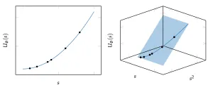
These basis functions are generally nonlinear functions of the state $s$, combined into a vector function $\boldsymbol{\beta}(s)$ or $\boldsymbol{\beta}(s, a)$. Even though the model is linear with respect to the basis functions, the resulting approximation can be nonlinear with respect to the underlying state $s$.

This is a great example of lifting features into a higher dimension (“升维”). In the left plot, the value is nonlinear with respect to the state $s$. However, in a higher-dimensional space formed by basis functions ($s$ and $s^2$), we can fit a flat plane to the data.

📁Example

Suppose the ground truth value function is $U(s) = s^2$.

From the table above, we see that the value function is nonlinear with respect to the state $s$. However, if we tailor our feature representation properly, say

Then the learnable parameter $\boldsymbol{\theta}$ could be $\boldsymbol\theta = [0,\ 0,\ 1]^\top$. In this case, our model $U_\theta$ perfectly captures the ground truth $U(s)$. For example, when $s=2$, we have

This exact fit can only be achieved when 2 conditions are met:

• ✅ we choose an appropriate feature representation. i.e., $\boldsymbol\beta(s) = [1,\ s,\ s^2]^\top.$
• ✅ we identify the right parameters. i.e., $\boldsymbol\theta = [0,\ 0,\ 1]^\top$

But what if we don’t choose an appropriate representation? Suppose our feature vector only includes linear terms:

If we use the least squares method to fit the parameter, we get $\boldsymbol\theta = [-1,\ 3]^\top$ (meaning $U_\theta(s) = -1 + 3s$).. In this case, the true value can not be perfectly approximated.

This is the most common case we encounter in real life.

⛳Objective

Now we know what $\boldsymbol\theta$ and $\boldsymbol\beta$ are, let’s see how to use the least squares method to solve for $\boldsymbol\theta$. Given $m$ states $s_{1:m}$ and their target utilities $u_{1:m}$, our objective is to minimize the sum of squared errors between the predicted value $\hat{U}_{\theta}(s_i)$ and the target value $u_i$:

We construct a feature matrix $\mathbf{X}$ where each row $i$ is the transposed feature vector for state $s_i$:

where $\boldsymbol{\beta}(s_i)$ is a column vector and $\boldsymbol{\beta}(s_i)^\top$ is a row vector.

Since the dot product of two vectors is symmetric ($\boldsymbol{\theta}^\top \boldsymbol{\beta}(s_i) = \boldsymbol{\beta}(s_i)^\top \boldsymbol{\theta}$), each prediction $\boldsymbol{\theta}^\top \boldsymbol{\beta}(s_i)$ is simply the $i$-th row (entry) of the matrix-vector product:

$\mathbf{X} \boldsymbol{\theta}.$

Let’s use a toy example to illustrate this:

• we have $m = 3$ samples of state
• feature vector is $\boldsymbol{\beta}(s) = \begin{bmatrix} 1 \\ s \end{bmatrix}$
• weight vector is $\boldsymbol{\theta} = \begin{bmatrix} \theta_1 \\ \theta_2 \end{bmatrix}$

Clearly, the last row is $[1, 2]$, so our feature matrix $\mathbf{X}$ is:

$\mathbf{X}=\begin{bmatrix} 1 & 0 \\ 1 & 1 \\ 1 & 2 \end{bmatrix}.$

Multiplying $\mathbf{X}$ by $\boldsymbol{\theta}$ gives all predictions at once:

Let’s verify with $i=3$. The prediction $\boldsymbol{\theta}^\top \boldsymbol{\beta}(s_i)$ becomes $\boldsymbol{\theta}^\top \boldsymbol{\beta}(s_3)$:

This is the exact last entry of the product $\mathbf{X}\boldsymbol{\theta}$.

Look back at our objective function:

If we define the error vector as $\mathbf{e} = \mathbf{X}\boldsymbol{\theta} - \mathbf{u}$, summing the squared entries of vector $\mathbf{e}$ is the same as taking its dot product with itself, $\mathbf{e}^\top \mathbf{e}$. Therefore, the equation above becomes:

✏Solution

Because this is a least squares problem, the minimum occurs where the derivative with respect to $\boldsymbol{\theta}$ is 0. Too see this intuitively, let’s first look at the 1D scalar version:

$J(\theta) = (x\theta - u)^2,$ assuming $x\neq0$. We have

The matrix calculus works the same way. Taking the gradient with respect to $\boldsymbol{\theta}$ and setting it to zero gives:

This gives Equation 8.16 in ADM

Depending on $\mathbf{X}$, we have 2 cases to consider:

• 1️⃣ when $\mathbf{X}^\top \mathbf{X}$ is invertible (i.e., $\mathbf{X}$ has full column rank): the $(\mathbf{X}^\top \mathbf{X})^{-1}\mathbf{X}^\top$ and the pseudoinverse $\mathbf{X}^+$ are mathematically identical. Case closed.
• 2️⃣ when $\mathbf{X}^\top \mathbf{X}$ (e.g., we have fewer states than features, resulting in a wide matrix): $(\mathbf{X}^\top \mathbf{X})^{-1}$ does not exist. Instead, we find $\mathbf{X}^+$ directly using SVD, which gives the minimum norm least squares solution.

Tip

In Python, numpy.linalg.pinv uses SVD behind the scene.

Therefore, whether $\mathbf{X}^\top \mathbf{X}$ is invertible or not, the safest and most general formula is:

$\boldsymbol{\theta} = \mathbf{X}^+ \mathbf{u},$

where $\mathbf{X}^+$ is the pseudoinverse of matrix $\mathbf{X}$. The pseudoinverse is often computed by first finding the singular value decomposition,

$\mathbf{X} = \mathbf{U}\mathbf{\Sigma}\mathbf{V}^*.$

We then have

That wraps up how linear regression can be used to approximate a value function!