Derive the Exponential Map for Rotation via Simple Physics

In A Mathematical Introduction to Robotic Manipulation, a 3D rotation is represented using an exponential map:

R(\omega, \theta)= e^{\hat{\omega}\theta} \in SO(3),

where

$\omega\in\mathbb{R}^3$ is a unit vector representing the rotation axis;
$\theta$ is the rotation angle, measured in radians;
$\widehat{\omega}$ is the skew-symmetric matrix associated with $\omega$ ;
$SO(3)$ is the special orthogonal group for all $3\times3$ rotation matrices such that $SO(3)=\Set{R\in\mathbb{R}^{3\times3}\mid R^TR=I,\ \det(R)=1}$

Here’s the question: rotation itself is easy to understand, but why on earth would anyone use the exponential function $e$ to represent it??🫣

Where does this equation come from, and how do we know that it really produces a rotation matrix?

In this post, I will try to answer these questions step by step.

Euler’s Theorem

Let’s first take Euler’s rotation theorem as given:

Any orientation $R \in SO(3)$ is equivalent to a rotation about a fixed axis $\omega \in \mathbb{R}^3$ through an angle $\theta \in [0,2\pi)$ .

We assume that $\omega$ is a unit vector:

|\omega|=1.

Using this theorem, we can imagine the following rotation:

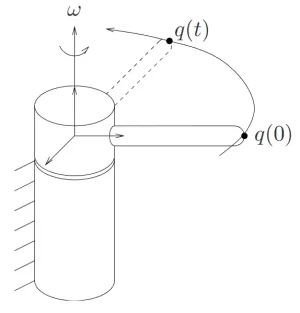
The $q(t)$ is a position vector representing the position of a point attached to the rotating body. As the body rotates, the tip of $q(t)$ moves in a circle around the axis $\omega$ .

Remark

For now, we assume that the rotation axis passes through the coordinate origin.

The Velocity of a Rotating Point

From high-school physics or The Feynman Lectures on Physics , we know that the velocity of a point moving in a circle is tangent to the circle (circular motion).

Suppose the rotation angle is $\theta(t)$ and the body rotates at a constant unit angular speed

\dot\theta(t)=1.

The velocity of the point is the cross product of the angular velocity and its position. Since the angular speed is $1$ , this simplifies to:

\dot q(t) = \dot\theta(t)=\omega \times q(t),

where $\times$ denotes cross product.

From a Cross Product to a Matrix

Instead of writing

\dot{q}(t) = \omega \times q(t),

we can represent the cross product using a skew-symmetric matrix:

\dot{q}(t) = \widehat{\omega} q(t).

Example

The $\widehat{\omega}$ is trivial once we see its components.
Suppose $\omega=\begin{bmatrix}\omega_1\\ \omega_2 \\ \omega_3\end{bmatrix}$ . Converting this to a skew-symmetric matrix gives $\widehat{\omega} = \begin{bmatrix} 0 & -\omega_3 & \omega_2 \\ \omega_3 & 0 & -\omega_1 \\-\omega_2 & \omega_1 & 0\end{bmatrix}.$

Remark

The hat operation does not change the physical meaning of $\omega$ . It simply converts the operation “take a cross product with $\omega$ ” into matrix multiplication.

Tip

Why is this conversion useful?
The idea is a shift in mindset. We move from vector-level cross product to matrix algebra. Suppose we need to calculate this:
$v = (a \times b) + (c \times b),$
and we can change it to
$\begin{align}v &= \widehat{a} b + \widehat{c} b \\&= \big( \widehat{a} + \widehat{c} \big)b\end{align}$
In the matrix world, we can leverage the computers to perform matrix calculation. ^248829

We now have $\dot{q}(t) = \widehat{\omega} q(t).$ What comes next?

Remark

Hint: this is a linear differential equationof the form $\dot{x}=Ax$ .

A Scalar Warm-Up

This is a good time to review the antiderivative.

The $\dot{q}(t) = \widehat{\omega} q(t)$ is actually no different from the scalar differential equation

$\dot{x}=ax,$

where $a$ is a scalar. Assuming $x>0$ , we see that

\begin{align} \dot{x} &= ax \\ \frac{dx}{dt} &= ax \\ \frac{1}{x}dx &=a dt \\ \int \frac{1}{x}dx &= \int a dt \\ \ln{|x|} &= at+C \end{align}

where $C$ refers to constant of integration.

Now, take the exponential of both sides:

\begin{align} e^{\ln{|x|}} &= e^{at+C} \\ |x| &= e^{at}\cdot e^{C} \end{align}

Since the exponential function $e$ is always positive, hence we can simplify as

x(t) = e^{at}\cdot e^{C}

The next steps is to determine the constant $e^C$ . A natural approach is to set $t=0$ , and we get

\begin{align} x(0) &= e^{0}\cdot e^{C} \\ e^{C} &= x(0)\\ \end{align}

Therefore, for the $\dot{x}=ax$ , the solution is

x(t) = e^{at}\cdot x(0)

Tip

The exponential appears because it has a special property: differentiating it reproduces the same function multiplied by the constant $a$ : $\frac{d}{dt}e^{at}=ae^{at}.$ That is exactly the behavior required to solve $\dot x=ax$ .

From the Scalar Exponential to Rotation

Informally, we can apply the exact same logic from our scalar solution,

x(t)=e^{at}x(0)

to our matrix equation:

$\dot{q}(t) = \widehat{\omega} q(t).$

Since $\widehat{\omega}$ is a constant matrix, the solution takes the same form

q(t) = e^{\widehat{\omega}t}\cdot q(0).

Remark

This is an intuitive way of looking at it. For a more rigorous reasoning, we have to go through matrix exponential, which I have decided to skip in this post.

At a unit angular speed, rotating for $t=\theta$ seconds produces a rotation of $\theta$ radians. Therefore,

q(\theta)=e^{\widehat{\omega}\theta}q(0).

The matrix that maps the initial position $q(0)$ to the rotated position $q(\theta)$ is thus

\boxed{ R(\omega,\theta)=e^{\widehat{\omega}\theta} }.

The preceding equation is still quite abstract and not easy to compute. The final piece of the puzzle is using Rodrigues’ rotation formula to convert the exponential map into a rotation matrix:

$R=e^{\widehat{\omega}\theta} = I + \widehat{\omega}\sin\theta + \widehat{\omega}^2(1 - \cos\theta).$

The Complete Picture

We can now connect all the pieces👏:

Euler’s rotation theorem tells us that every 3D orientation can be described by an axis $\omega$ and an angle $\theta$ .
A point rotating about that axis satisfies a velocity equation involving the cross product.
The cross product can be written as multiplication by the skew-symmetric matrix $\widehat{\omega}$ .
This produces the linear differential equation $\dot q(t)=\widehat{\omega}q(t).$
The solution of that differential equation is $q(t)=e^{\widehat{\omega}t}q(0).$
Rotating through an angle $\theta$ therefore gives $R(\omega,\theta)=e^{\widehat{\omega}\theta}.$
Because $\widehat{\omega}$ is skew-symmetric, the resulting matrix belongs to special orthogonal group $SO(3)$ .

Final remarks

$\widehat{\omega}\in\mathfrak{so}(3)$ , where so(3) is the vector space of all real $3\times3$ skew-symmetric matrices.

$e^{\widehat{\omega}\theta}\in SO(3)$ is a finite rotation matrix.

The vector $\omega\theta\in\mathbb{R}^3$ contains the exponential coordinates of rotation.

The direction of $\omega\theta$ gives the rotation axis, while its magnitude gives the rotation angle.

The exponential map connects an instantaneous rotational velocity in $\mathfrak{so}(3)$ to a finite rotation in $SO(3)$ .

The main idea is therefore:

\boxed{ \text{constant rotational velocity} \quad\xrightarrow{\text{integrate over time}}\quad \text{finite rotation} }

The matrix exponential is simply the mathematical operation that performs this integration.

Derive the Exponential Map for Rotation via Simple Physics

Euler’s Theorem

The Velocity of a Rotating Point

From a Cross Product to a Matrix

A Scalar Warm-Up

From the Scalar Exponential to Rotation

The Complete Picture

See also...