If you have ever used physics simulators like Isaac Sim, ManiSkill, or Overview - MuJoCo Documentation, you have likely encountered the term PD controller.
If you’ve worked with hardware libraries like libfranka: C++ library for Franka Robotics research robots, you might have also noticed parameters like, “stiffness”, “damping”.
In this post, I want to share a practical, intuitive understanding of this topic, bridging the gap between control theory and robot learning.
RemarkUnless otherwise stated, the mathematical notation in this post follows Russ Tedrake’s conventions in Robotic Manipulation.
The Math Expression
Let’s start by looking at the math. A standard PID controller is expressed as:
In practical robotics, we almost always drop the integral ("") term. Accumulating past errors can lead to dangerous, unpredictable movements in contact-rich tasks (a phenomenon known as integral windup). This simplifies our equation to a PD controller:
where
- : the command sent to the actuator (pulse-width modulation), simplified here as torque
- : the current actual joint position
- : the desired joint position (target)
- : the position error
- : the current actual joint velocity
- : the desired joint velocity (target)
- : the velocity error
- : the proportional gain (think of this as stiffness or a “spring”).
- : the derivative gain (think of this as damping or “friction”).
RemarkIn multi-joints robot, and are technically diagonal matrix, but treating them as scalar values works perfectly for building intuition!
RemarkIn control theory, it is related to mass-spring-damper model.
The Franka Example
Let’s step away from the equations and look at an example I made using Franka Research 3.
When I use JointPositionControl in libfranka to move a robot, there are two levels of control happening simultaneously.
📌The High Level (trajectory generation)
First, I used trajectory generator like (like ruckig: Motion Generation for Robots and Machines) to create a smooth path that respects the limits of velocity, acceleration, and jerk. This trajectory matches the Franka’s 1KHz control frequency. Every millisecond (), we generate 7 new desired joint position values:
- ,
- ,
- ,
// ⭐️control runs every 1ms
robot.control([&](...) -> franka::JointPositions {
//...
franka::JointPositions pos = {/* 7 target joint values */};
return pos;
});RemarkIf you want to know more about the joint position notation, see Understanding Franka Robot Control Parameters.
RemarkIf you want to know more about how I control the Franka, see frankz.
📌The Low-Level (Hardware Control)
At the hardware level, the PD controller takes over. The pos I return in the C++ code becomes the desired joint position .
The robot’s internal controller calculates the required torque:
The libfranka hides this high-frequency loop from us. We feed it targets(desired joint position), and the internal PD controller tracks them.
Example: One Joint, One Step
Let’s walk through a simple one-joint scenario to see how and interact.
📌0. Setup
- Current state: ,
- Target state: ,
- Gains: ,
📌1. Compute Initial Torque
The “spring” () pulls the joint forward.
📌2. The World Dynamics
The joint accelerates. As increases, the position error shrinks, reducing the torque. The joint eventually decelerates and settles at the target.
📌3. Braking
Imagine the robot is almost at the target (), but it’s moving way too fast (). What happens?
The torque is heavily negative! This means the robot is braking. The “D” term () acts as a damper to slow the robot down and prevent it from overshooting the target.
Why does the ?In pure joint position control, we often treat the desired velocity at the exact target as zero so the robot comes to a rest.
Analogy: choose either
franka::JointPositionsorfranka::JointVelocities.
With this example, we build an intuition on the and .
- (Spring): Pulls the robot toward the target.
- (Damper): Slows the robot down to prevent overshooting.
Exercise 1
Assume we have
Calculate the torque for the following scenarios:
| (a) | 1.0 | 0.0 | ? |
| (b) | 1.2 | 2.0 | ? |
| (c) | 0.0 | -5.0 | ? |
🗣Answer (a)
The robot is at the target and not moving. No actuation needed.
🗣Answer (b)
The robot has overshot the target and is still moving away from it. The controller aggressively pulls it back and brakes.
🗣Answer (c)
The robot is far from the target and currently moving in the wrong direction (negative velocity). Both the spring and the damper work together to aggressively push it forward.
PD Control in Robot Learning
When we transition to robot learning, things get interesting. A neural network policy () rarely outputs raw torques. Instead, it outputs commands in a specific action space.
Take ManiSkill, for example. It offers several controllers:
pd_joint_delta_pospd_ee_delta_pospd_joint_vel- …
So how does the action spaces work?

- (
pd_joint_delta_pos): The policy outputs a small action . The target becomes . The neural network is directly adjusting individual joint angles. - (
pd_ee_delta_pose): The policy outputs a desired change in the [end-effector] pose (a SE(3)). An inverse kinematics solver() converts this desired EE pose into target joint positions(). - (
pd_joint_vel): The policy directly outputs the joint velocities.
TipThe choice of controller defines the action space your policy sees.
| Controller | Action dim | Policy outputs | Easier for Robot Learning? |
|---|---|---|---|
pd_joint_delta_pos | 7 | Small joint deltas | ok |
pd_ee_delta_pose | 6 | position + rotation delta | easy |
pd_joint_vel | 7 | joint velocities | hard |
EE-space controllers are typically much more sample-efficient. The policy only needs to learn “move gripper left 10cm,” rather than learning the complex kinematics required to coordinate 7 individual joints to achieve that same leftward motion.
Exercise 2
💬Question(1) You’re training an RL policy for a peg-in-hole task. The peg needs to safely comply with contact forces when it hits the edge of the hole. Which gains do you want?
- (A) High Low
- (B) Low Low
- (C) Low High
RemarkThe “peg-in-hole” is the problem of inserting a (round) peg into a (round) hole.
©️Samuel Hunt Drake, “Using compliance in lieu of sensory feedback for automatic assembly.”, PhD thesis, Massachusetts Institute of Technology, 1978.
🗣Answer (1)
The answer is B. To elaborate, I want you to imagine 2 things.
- high 📈: iron grip, stiff spring, robot fight back when hitting hole edge
- low 📉: gently, soft spring, robot yields, slide in when hitting hole edge
TipThe solution to this task is impedance control.
💬Question(2) Your simulated Franka robot arm is oscillating wildly around its target position. What should you change?
- (A) Increase
- (B) Increase
- (C) Decrease
🗣Answer (2)
Increase . To be honest, I personally encountered this issue in practice. The end-effector is oscillating around a position and it seems vibrating. To solve this issue, we actually need a damper.
Here’s the intuition.
| Spring | Damper |
|---|---|
| overshoot, bounce back, over shoot = oscillation | spring but absorb, approach smoothly |
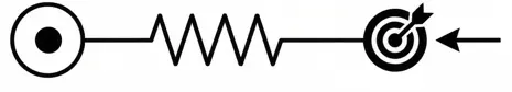 | 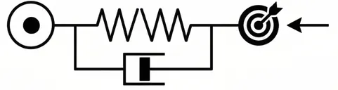 |
TipKey takeaway: Oscillating wildly? > You need MORE damping > INCREASE .
💬Question(3) You switch from pd_ee_delta_pos (3-dim) to pd_joint_delta_pos (7-dim) for the same pick-and-place task. Training now requires 5x more samples. Why?
🗣Answer (3)
The intuition behind is that the pd_joint_delta_pos must learn much more.
pd_ee_delta_pos | pd_joint_delta_pos | |
|---|---|---|
| dimension | 3 | 7 |
| action | move gripper left | move gripper left by moving joints 1-7… |
| learning objective | what to do | what + how(IK solver) |
It’s not just “more dimensions”. It’s that the policy must now learn the kinematics of the robot, which the IK solver was doing for free.
💬Question(4)
Imagine a 1D robot joint that should go to position , starting at . We have the following observations:
- behavior A: overshoots to , back to , then , slowly settles to
- behavior B: … reaches and stays perfectly, no overshoot
- behavior C: … slowly to , … , … , takes forever to reach
We have these gain settings:
- High Low
- Low Low
- Moderate High
Which behavior goes with which gains?
🗣Answer(4)
It turns out that in these are the terms in control theory:
- A: 1, High Low , underdamped, fast but risky, oscillation can damage your robot⚠️
- B: 3, Moderate High , critically damped, sweet spot
- C: 2, Low Low , overdamped, safe but slow, typically frustrates robot learning
💬Question(5) You’re training a policy with pd_joint_delta_pos. During evaluation, the robot arm moves way too slowly even though the policy outputs large actions. Which is more likely: is too high, or is too low?
🗣Answer(5): is too low. The spring is not strong enough to pull the joint to the target.
Summary
- PID controller = proportional + integral + derivative feedback loop. Robotics usually uses PD(drop the ).
- : is spring(pulls to target) and is a damper(prevent overshoot)
- tuning: high means stiff and fast but oscillation, high means smooth but slow. Sweet spot is moderate.
- robot learning: the policy outputs action. The choice of using which controller defines the action space!
delta_posvstarget_delta_pos: the former resets from the current state (forgiving) while the latter accumulates (precise but risky)- why no term? It causes windup in contact-rich tasks.