As part of my Homework 1: Imitation Learning for CS 185/285: Deep Reinforcement Learning and my research in robot learning, I needed to quickly get up to speed on the basics of Flow Matching. In my previous blog post, A Beginner’s Guide to Flow Matching, I explained the core intuition behind the topic.
This post dives deep into applying flow matching to action chunking, specifically geared toward those wanting to understand the mechanics behind modern robot imitation learning. To respect academic integrity, I won’t release my source code. Instead, I’ll explain the architecture and the math from a big picture perspective.
What is Action Chunking?
Let’s first review the concept of action chunking, popularized by research like 📄Learning Fine-Grained Bimanual Manipulation with Low-Cost Hardware (ACT). In the standard imitation learning, the policy is defined as:
The policy represents a probability distribution over a single action conditioned on the current observation . Instead of predicting just one single action , the action chunking proposes predicting a sequence, or chunk, of future actions all at once:
where is a fixed -length sequence of actions.
RemarkThe creates an open-loop execution phase: the environment will receive the action from agent at time , then at time , and so on until . The agent will query observation again on time .
As a concrete example, consider the Push-T task from 📄Diffusion Policy: Visuomotor Policy Learning via Action Diffusion, where a robot agent pushes a T-shaped block into a target region.
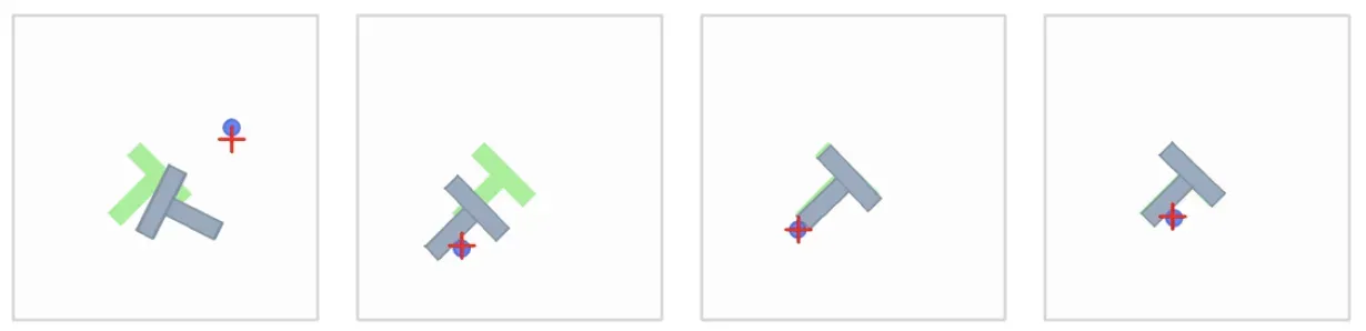
The Push-T environment.
In this task, the observation relies on low-dimensional state vectors rather than high-dimensional images (i.e., we use a state instead of a visual observation ). The state is a 5-dimensional vector containing:
- -coordinate of the agent
- -coordinate of the agent
- -coordinate of the T-block
- -coordinate of the T-block
- (rotation angle) of the T-block
The action is a 2-vector dictating the agent’s target position.
RemarkFor the distinction between (fully observed) and (partially observed), you can refer to Why the Gymnasium API Looks the Way It Does?.
Why Flow Matching?
The simple answer: generative models like flow matching and diffusion models are more expressive than a mixture of Gaussians.
RemarkChelsea Finn refers to applying generative models in imitation learning as an “advanced version of imitation learning,” while Sergey Levine states that using generative models in imitation learning solves the issues of naive behavioral cloning. For a more in-depth discussion, I’ve written a separate post: Why Naive Behavioral Cloning Doesn’t Work?.
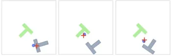
As an example, in the Push-T environment, a policy powered by a generative model can learn to approach the T-block from the left or from the right.

©️Chi, et al.
With a mixture of Gaussians, “the action to the left” averages with “the action to the right” and produces “go straight” — which is not what we want.😅
The Dataset: From Episodes to Training Samples
Expert demonstrations are recorded as episodes of varying lengths, depending on how long it took the expert to solve the task. To avoid jagged arrays during training, all episodes are concatenated into flat arrays. An episode_ends array marks the boundary indices of each episode.
For example, consider two short dummy episodes:
We concatenate their actions and states into flat vectors:
The episode_ends array is [5, 12], meaning Episode 0 spans indices 0-4, and Episode 1 spans indices 5-11. With a chunk_size of , a sliding window extracts (state, action_chunk) pairs. Each training sample pairs one state with the next consecutive actions.
💬Question: Given the episodes above and , what are the valid starting indices? Why are indices 3 and 4 excluded for Episode 0?
🗣Answer: The valid starting indices would be [0, 1, 2, 5, 6, 7, 8, 9]. Indices 3 and 4 are excluded because they don’t have actions left before the episode ends. The same logic applies to Episode 1, where index 10 is excluded.
Episode 0:
[a0] [a1] [a2] [a3] [a4]
 ✓    ✓    ✓    ✗    ✗
 0    1    2    3    4
💬Question: During training, the dataloader shuffles and mixes samples from different episodes within a batch. Why is this acceptable?
🗣Answer: Because the underlying task remains constant. Every (state, action_chunk) pair is a self-contained snapshot of an intermediate step toward the same objective. Drawing randomized, uncorrelated transitions across different demonstrations also ensures the batch has high entropy, which improves gradient quality.
Training: What the Network Sees
In Flow Matching, we define a continuous flow from a simple noise distribution to our complex data distribution. Let’s establish our notation. Let the expert action chunk be our target data , and let be a sample of pure noise.
We introduce a flow-time variable .
RemarkWe use to represent the integration time of the flow, keeping it distinct from , which represents the environment timestep.
During a training step, the network receives the current state , a specific flow-time , and an interpolated action chunk . We construct this straight-line interpolation as:
The network’s objective is to predict the velocity (the derivative with respect to ). For a straight-line optimal transport path, the exact target velocity is simply:
RemarkBecause during training, the (expert action chunk) and (initial action chunk) are constant.
TipCrucially, the network never sees the raw expert chunk as an input. It only sees the noisy intermediate state and learns the direction to push it toward reality. Therefore, the network is denoted as (velocity) rather than .
For example, if the chunk size , then the dimension of the input of the network would be
state(5) + interpolated_chunk(2 * 3) + tau(1) = 12
and the output would be a velocity vector of dimension
action_dim(2) * chunk_size(3) = 6
💬Question: The target velocity () does not depend on . Why does still matter as an input to the network? What would go wrong if we always set during training?
🗣Answer:
The target velocity is constant, but the location in the vector field is constantly changing. We are training the network to predict the correct velocity from any coordinate along the path.
If we only trained on , the network would only learn how to predict velocities when looking at pure noise. During inference, after taking the first integration step, the data becomes partially denoised (). The network would have no idea how to handle this new, structured input, and the integration would immediately collapse.
💬Question: At , the network input is pure noise. At , it is almost the exact expert data. At which extreme is the prediction task hardest?
🗣Answer: It is hardest at . The network is looking at complete static and has to guess the exact trajectory toward a highly specific, structured action chunk.
Inference: Euler Integration
At inference time, we do not have access to expert data. We start by sampling pure noise and use the learned velocity field to integrate forward using the Euler method.
If we choose num_steps = 4, our step size is 1 / 4 = 0.25, i.e., . The integration process looks like this:
| Step | Current | Velocity Input | Next chunk |
|---|---|---|---|
| 0 | 0.00 | Pure Noise | Chunk at |
| 1 | 0.25 | Partially denoised | Chunk at |
| 2 | 0.50 | Mostly structured | Chunk at |
| 3 | 0.75 | Highly structured | Final Action Chunk () |
💬 Question: Why is the network never evaluated at during inference?
🗣Answer: Because the Euler step taken at pushes the chunk exactly to the boundary of . Once we arrive at the destination, the flow is complete, and we extract the actions to execute.
TipThis mirrors how we train the model: we sample from a uniform distribution . We don’t train on because the velocity field doesn’t need to push the data anywhere once it has arrived.
💬 Question: What happens if you set num_steps = 1? Under what condition would a single step produce a perfect sample?
🗣 Answer: Setting num_steps = 1 means taking one massive Euler step:
This would only produce a perfect sample if the network learned the exact true velocity () flawlessly. Because Flow Matching paths are straight lines by construction, a perfect velocity prediction means one step is theoretically sufficient. In practice, predictions at are the noisiest, so breaking the flow into smaller steps allows the network to correct its course as the chunk becomes more structured.
Reflections
Why operate on the full chunk?
Flow matching doesn’t predict a single action. It generates an entire chunk of future actions at once. The noise, interpolation, and velocity all operate on the full flattened chunk vector.
💬Question: What advantage does this give over predicting each action in the chunk independently?
🗣Answer: It allows the model to learn temporal correlations across time steps. If action initiates a rightward push, action must logically follow through. Operating on the full chunk allows the velocity field to enforce physical consistency and smooth trajectories. Predicting actions independently would destroy this temporal coherence, leading to jerky, contradictory movements.
Multimodality
💬 Question: Imagine two expert demonstrations show “push left” and “push right” for the exact same state. How does Flow Matching mechanically produce both strategies? Where does the “choice” come from?
🗣 Answer: The choice comes entirely from the initial noise sampled at the start of inference.
If noise sample lands on one side of the latent noise space, the learned velocity field sweeps it toward the “push left” action chunk. If noise sample is drawn, it might land in a region that flows toward the “push right” chunk. The state is identical in both cases; the random starting point dictates the final mode. This is why generative models easily handle multimodality, whereas a standard MSE policy would simply average the two demonstrations, resulting in a useless “push straight” command.
How does the model learn the full velocity field?
During training, each dataset sample is paired with one random and one random noise vector per step. The model never sees the same sample tracked across all values in a single pass.
💬 Question: How does the model eventually learn the velocity field across the entire range?
🗣 Answer: The coverage of the flow-time is achieved over the course of multiple epochs. The training loop behaves like this:
Because the dataset is iterated over hundreds of times, a specific state will eventually be evaluated against many different values of and many different noise vectors . Over time, the network pieces together the complete continuous vector field.
Cross-episode shuffling
💬Question: The dataloader shuffles the dataset every epoch. Does “shuffle” mean rearranging chunks within a single episode, or across all episodes?
🗣Answer: It shuffles across all episodes since each pair is self-contained. A single batch freely mixes samples from different demonstrations:
Batch: indices[7], indices[1], indices[5]
     =       8,          1,          6
     → (s8, [a8,a9,a10]),  (s1, [a1,a2,a3]),  (s6, [a6,a7,a8])
       ^^^ from ep1          ^^^ from ep0       ^^^ from ep1